Zoran Čučković
[ This page is archived for consistency: see the new version on LandscapeArchaeology.org. ]
Current plugin version: 0.5
It took me long time to develop an algorithm for the visibility analysis which would be comparable in terms of speed and quality to those available in other packages. And then some more time to tweak it for the type of analysis the QGIS visibility plugin is intended: higher volume calculation of multiple viewsheds over standard (coarse) elevation models. But here it is - an implementation which is faster than previous ones by a factor of 10 (at least).
1. Performance test
There is a set of data files in plugin’s repository for testing purposes: a shapefile with several hundred observer points (462 to be precise) and an elevation model extracted from SRTM DEM, with 90 metres resolution (see resources below). All analyses were made using following parameters: a radius of 5000 metres for each point and eye level of 1.6 metres above ground. For ArcGis the standard viewshed module with multiple points was used (ref. below), and for QGIS plugin the cumulative visibility option.
My laptop has 8 Gb of working memory and 2.4 GHz processor. I’ve never touched RAM allocation for software I use - perhaps it would run faster with some tweaks - but the overall picture on the table below seems clear.
| 5 x test | ArcGis 10.1 viewshed | QGIS viewshed plugin 0.4 | QGIS viewshed plugin 0.5 |
| Maximum | 52,0 | 56,1 | 3,6 |
| Minimum | 47,2 | 53,3 | 4,2 |
| Average (all in seconds) |
49,5 | 54,3 | 3,8 |
So, upon five tests the new 0.5 version is faster than ArcGis by a factor of ten. In fact, only the standard multiple visibility as available in ArcGis was tested, which is a visibility model that contains only true/false values - if we were to perform some additional steps to obtain a cumulative result (a sum of rasters), the analysis time would probably be somewhat longer.
Anyway, the result is sweet, isn’t it? But, is there a catch, you may wonder … I will not go to all details (I’m still not sure if and how this might be published), but the basics of the algorithm used are explained below.
2. Algorithm
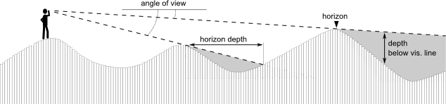
Fig. 1 Line of sight anatomy.
Pixel-centric approach
Implemented algorithm casts an array of lines-of-sight from the observation point to the perimeter of the analysed area. The position above or below the visibility line is then recorded for each pixel encountered along the line. Note that these lines do not necessarily touch the centre of each pixel (Fig. 2) - the height values are therefore interpolated between pairs of pixels on each side of line-of-sight (linear interpolation).
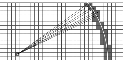
Fig. 2 Ray casting algorithm.
In order to simplify the procedure, observer and target point locations are approximated to the pixel centre. This may seem problematic since even sub-pixel variations of the observer point could have perceptible impacts on the final output. However, susceptibility to variations within the immediate observer vicinity is an inherent problem of viewshed modelling in general, regardless of the algorithm used (see above). What is more, if our observer is a living being, some kind of movement and adaptation should always be expected: these very variations might be turned into his/her/its advantage. We need flexibility much more than precision. In any case, a finer DEM should be used (even if resampled) in order to obtain more detailed results with any viewshed algorithm. Otherwise, one may question the significance of differences in obtained results when these are due to sub-pixel shifts of the observer location, i.e. below the precision of the DEM used.
The density of the lines of sight per pixel is apparently diminishing with the distance from the observer point, implying less possibility to choose the most appropriate one for testing pixel’s visibility (i.e. the ray closest to the centre of the pixel). That error is illustrated on Fig. 3 (which makes a nice “squaring of the circle” fractal). The perimeter to which rays are cast is of square shape (as of version 0.5) and the final, circular, output is produced by clipping off values beyond specified analysis radius.
(Note that the horizontal shift does not affect the calculation of intervisibility lines which is made from the centre observer’s pixel to target pixel centre.)
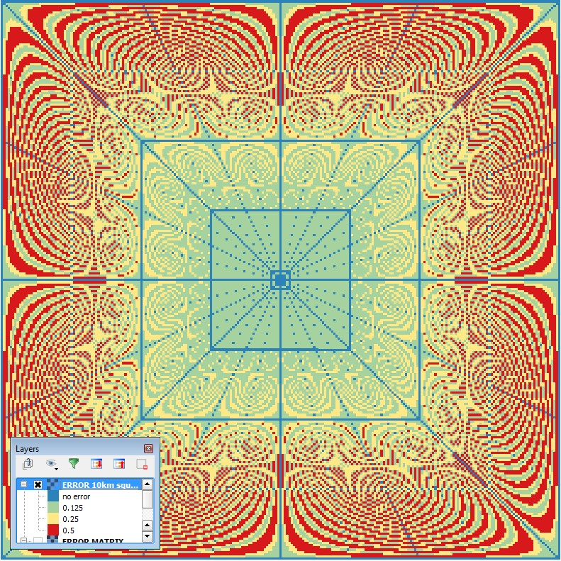
Fig. 3 Shift of the nearest line of sight from each pixel centre.
What becomes apparent when looking at the error matrix on Fig. 3 is that errors higher than a quarter of a pixel (red) stay out of the large square which happens to cross half of the radius. (maximum possible error is half pixel size, 0.5.) Likewise, errors higher that an eighth of a pixel (yellow) stay outside the square at the quarter radius distance. This comes handy for estimating the accuracy of the viewshed calculation: 1/4 radius = very good, 1/2 radius = good, above 1/2 radius = not-that-good. Now, in some cases the last one may indeed be “bad”, for instance when trying to estimate depth below visible horizon (invisibility) more accurately. For such cases it is possible to artificially double the radius by choosing “fine” algorithm. The result will be clipped back to the specified radius and will now be devoid of errors above quarter of a pixel.
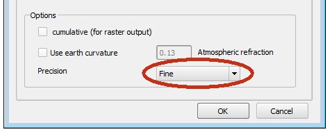
Fig. 4 Option fine
Some inconsistencies may arise in the “red zone” when calculating visible horizon. The horizon is composed by selecting the farthest visible pixel for each line of sight. When only a couple of lines is available per pixel, some ambiguities may arise. The pixel to the left on Fig. 5 should be selected, but upon first visit it’s not visible because of the interpolation of height with its (lower) neighbour, while upon the second visit the line of sight hits an even farther visible pixel to the right. This problem can be avoided by using the fine algorithm option or by increasing the radius of analysis.
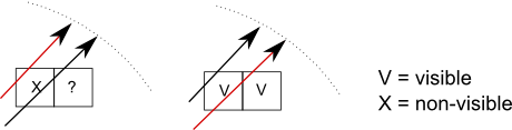
Fig. 5 The ambiguity when selecting horizon pixel.
3. Errors !?
So, the algorithm is fraught with errors - not a pleasant thing to hear! … and for that reason you don’t hear much about it concerning other implementations. To have a better grasp on the volume of ‘errors’ in viewshed modelling, it suffices to run an analysis in different software packages (provided different algorithms are used). [cf. Fisher 1993 for such an exercise with an in depth discussion]. The size of inconsistencies is easily discernible on Fig. 6a-b. There is a whole cluster of visible areas appearing in ArcGIS model only, while the GRASS r.los model seems to disagree markedly with the one produced by our algorithm. How can that be?
Note that the observer point (blue) is very close to the invisible area, and that the inconsistencies arise after a large black gap. This indicates that the problem most probably lies in interpolation of height values between pixels in the observer’s vicinity. These minute inconsistencies get particularly amplified because of closeness to the observer. In fact, the horizontal line of sight shift affecting the outer zone of the viewshed (Fig. 3) is much less significant (or even insignificant) when compared with the height interpolation (or sampling) method.
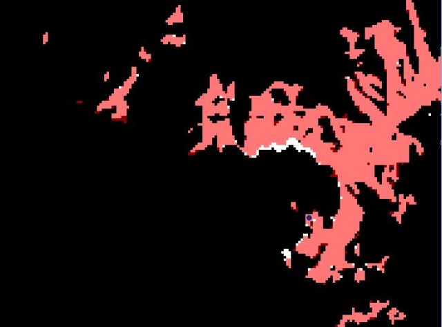
Fig. 6a Implemented algorithm (white) overlaid with GRASS r.los model (red).
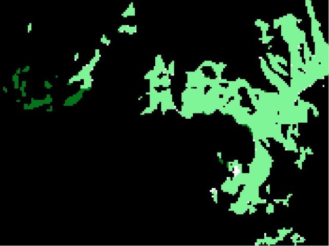
Fig. 6b Implemented algorithm (white) overlaid with ArcGIS 10.1 viewshed model (green).
Resources:
Datasets used: GitHub repository.
References
ArcGis viewshed module documentation.
Fisher, P. (1993). Algorithm and implementation uncertainty in viewshed analysis. International Journal of Geographical Information Science 7 (4), 331-347.
Kaučič, B. and Žalik, B. (2002). Comparison of Viewshed Algorithms on Regular Spaced Points. SCCG ‘02 Proceedings of the 18th Spring Conference on Computer Graphics, 177-183. [www.cs.swarthmore.edu/~adanner/cs97/f06/ps/Viewshed.ps]